Lab 10 -- Off Line Springs
Lab 10 (click here
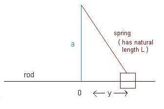
for pdf) is about: "a box of mass m sliding along a frictionless rod, is
attached to a spring of natural length L by a pivot...." Read the last page
of the lab (see the above link) to understand where this system comes from. If
you understand the that the more unnaturally stretched / compressed the spring
is, the more force it exerts, the system makes sense. The box is
"unnaturally stretched or compressed" if the actual length of the
spring differs from the natural length, L.
Actual length of spring = sqrt(a^2+y^2) [see below]
Natural length of spring = L.
See the handout to see how one would derive M*y'' = K_s(-y + L*y / sqrt(y^2+a^2) ).
For M = L = K_s = 1, we have
y'' = -y + y / sqrt(y^2+a^2). (1)
On to the problems:
- Rewrite Equation (1) above as a first order system. Then show that if this
system is at equilibrium [i.e. y' = y'' = 0] and a >= 1, then y = 0.
Now explain why y = 0 is a stable equilibrium point. Is the spring compressed [actual length of string smaller than natural] or stretched [actual length of string bigger than natural]? Remember that
actual length of the spring = sqrt(a^2+y^2),
natural length of spring = L = 1.
If the spring is compressed, visualize such a system (as described on the back page) with a compressed spring. If it is stretched, visualize such a system (as described on the back page) with a stretched string. In particular, visualize the spring trying to get back to its natural length. - Find that there are three equilibrium points of the system above (three
y-values satisfying y'' = y' = 0), except that a < 1.
Draw diagrams like that on the back page of the handout for each equilibrium point. There will be one equilibrium point at y = 0, but this equilibrium point is unstable. Again, I would like an explanation of this in terms of the spring attempting to reach its natural length. - Assume 0 < a < 1. Linearize the system above near each
equilibrium point. This involves computing the partial derivatives of y and
y' at each equilibrium point by hand. Or maybe not. You might be thinking
that that's tedious Calculus I busywork that computers know how to do.
Here's how we can do that with a computer. Let y' = v. Notice that v'v = 0, and v0 = 0 (why?). Thus our linearized system around the equilibrium point (y0, v0) will be computed by the formula:
-------
y'linear(y0, v0) = y'(y0, v0) + v = v0 + v = 0 + v = v
v'linear(y0, v0) = v'(y0, v0)+ v'y(y0, v0)*(y-y0)+v'v(y0, v0)*(v-v0)
= v'(y0, v0) + v'y(y0, v0)*(y-y0)
-------
where (v0, y0) is the equilibrium point we are linearizing around. I wrote a couple lines of Matlab commands to compute the linearized v:
-------
maple('v_prime:= (y,v)-> -y+y/sqrt(a^2+y^2)')
maple('subs(y0=0, v_prime(y0,v0) + subs(v=v0,subs(y=y0,diff(v_prime(y,v),y)))*(y-y0))')
-------
The second command will return you v'linear around (y0, v0) for y0 = 0. (The first line defines "v_prime" as a function of y and v.) To linearize for the equilibrium points, you can replace the zero in purple in the second command with other equilibrium values of y0.
(Again, you are free to linearize this system by hand instead, but arithmetic errors will still cost you. One useful way to look at the behavior of this system would be to consider another form of the linearized system involving the Jacobian matrix [cf. p. 502]. This will involve some partial derivatives, but the Jacobian matrix can be used in the analysis of what type of equilibrium the point is [cf. pp. 503-504 of your text; pp. 376-380 may also help].)
Now that you have the linearization, determine what type of equilibrium point each is. - Follow the instructions here and make sure that the orbits you plot satisfy y(0) = 1. Give a couple sentences or more of explanation of what is physically happening for large and small initial velocity. Approximate to the nearest tenth the value of v0 at which the behavior changes.
- You'll modify the system you entered into pplane by adding a small amount of friction to it, say -.1*v. Remember to do the part concerning finding a v1, v2, v3, and v4.
- We'll be replacing the damping with an external force of magnitude .4*sin(w*t).
Pplane only deals with autonomous systems. Thus the main thing to do here is
make an m-file that ode45 can interpret. Make an m-file for ode45 that
models the system
y' = v
v' = -y + y / ((.5)^2+y^2)^.5 + .4*sin(w*t).
You'll plot the result of ode45 (or ode23) for different values of w. When you find a w where resonance seems to occur, print out this plot and record your value of w. (If you're uncertain about how to use ode23 to solve this kind of system, you can look back at the instructions for Exercise 4 of Lab 9.)
Note: Use plot(u(:,1), u(:,2)) to plot with y on the horizontal axis and v on the vertical axis (as in pplane).
(Further note: The lab handout says to plot(u(:,2),u(:,1)), which would plot v on the horizontal axis and y on the vertical axis ... but since phase portraits are typically y' vs y, not y vs. y', the order would better be switched.) - Now plot the same system, but with w = 0.1, for t in [0,300]. Describe the
behavior physically: does the orbit seem to settle on one of the two points?
Plot in a bigger interval (say, t in [0,3000]) and see whether your answer
seems to hold.
Remember to plot velocity against time. You may at some point want to use the command plot(t,u(:,2)) to do this. Indicate where acceleration seems greatest and to answer the question about the bug. - Just summarize your results by answering the questions given here.
That's it for Lab 10.